Difference between revisions of "GRA"
Jacandrade (talk | contribs) |
Jacandrade (talk | contribs) |
||
| Line 30: | Line 30: | ||
The input on the left allows the user to upload a file with the time series to be analysed. The file MUST be on a .CSV format to ensure compatibility with the forecasting algorithm, containing all the values in the first column, one value per row: | The input on the left allows the user to upload a file with the time series to be analysed. The file MUST be on a .CSV format to ensure compatibility with the forecasting algorithm, containing all the values in the first column, one value per row: | ||
| − | <code> | + | <code>value1</code> |
| − | value1 | ||
| − | value2 | + | <code>value2</code> |
| − | value3 | + | <code>value3</code> |
| − | value4 | + | <code>value4</code> |
| − | ... | + | <code>...</code> |
| − | </code> | ||
Each row represents a time point in the time series. You don't need to enter the month for the values, as each entry is considered a new point value for the month following its preceding value. The results will display the index value of each entry as ordered in the entry data in the X axis starting at 0, and the forecast results will be added as entries at the end of the time series original values. | Each row represents a time point in the time series. You don't need to enter the month for the values, as each entry is considered a new point value for the month following its preceding value. The results will display the index value of each entry as ordered in the entry data in the X axis starting at 0, and the forecast results will be added as entries at the end of the time series original values. | ||
| Line 52: | Line 50: | ||
The input on the left allows you to quickly create a forecast by pasting the values of a time series in the text box and using it as an input. Each value for the time series must be entered one after the other, separated by a semi-colon '';''. You will get an error message if any of the values are not in the correct format. Once everything is ready click the calculate button below the input to generate the forecast. You can copy and paste the example below in the tool for a demonstration: | The input on the left allows you to quickly create a forecast by pasting the values of a time series in the text box and using it as an input. Each value for the time series must be entered one after the other, separated by a semi-colon '';''. You will get an error message if any of the values are not in the correct format. Once everything is ready click the calculate button below the input to generate the forecast. You can copy and paste the example below in the tool for a demonstration: | ||
| − | < | + | <pre>2500;2750;1598;1777;2100;2107;2213;1993;1768;1479;1344;1389;1433;1477;1578;1611;1678;1587;1523;1124;1388;1299;1433;1399</pre> |
=== The results === | === The results === | ||
Latest revision as of 18:03, 5 August 2018
Contents
Growth Risk Analyser
Introduction
In the research phase of the project, simulation models were developed to analyse how changes in supply and demand affect production planning, economic performance, supply chain relationships, value added, potential product success, market trends and developments and thus competitiveness as measured by the updated FACI. One of the outcomes of the research is the Growth risk analyser tool, implemented through simulation/forecasting models for analysing and forecasting pricing trends in the short term: up to 12 months with a confidence band of 95% in the case of this tool. Forecasts given outside of 12 months become less reliable as the forecast horizon increases (up to 24 months are generated by the tool).
The tool analyses a time series of data of any value type such as profit per month, average sales quantity per day/week/fortnight/etc, average catch/landings per month/semester/year/etc, containing a minimum of 24 values (to ensure accuracy).
Tool Overview
Landing page
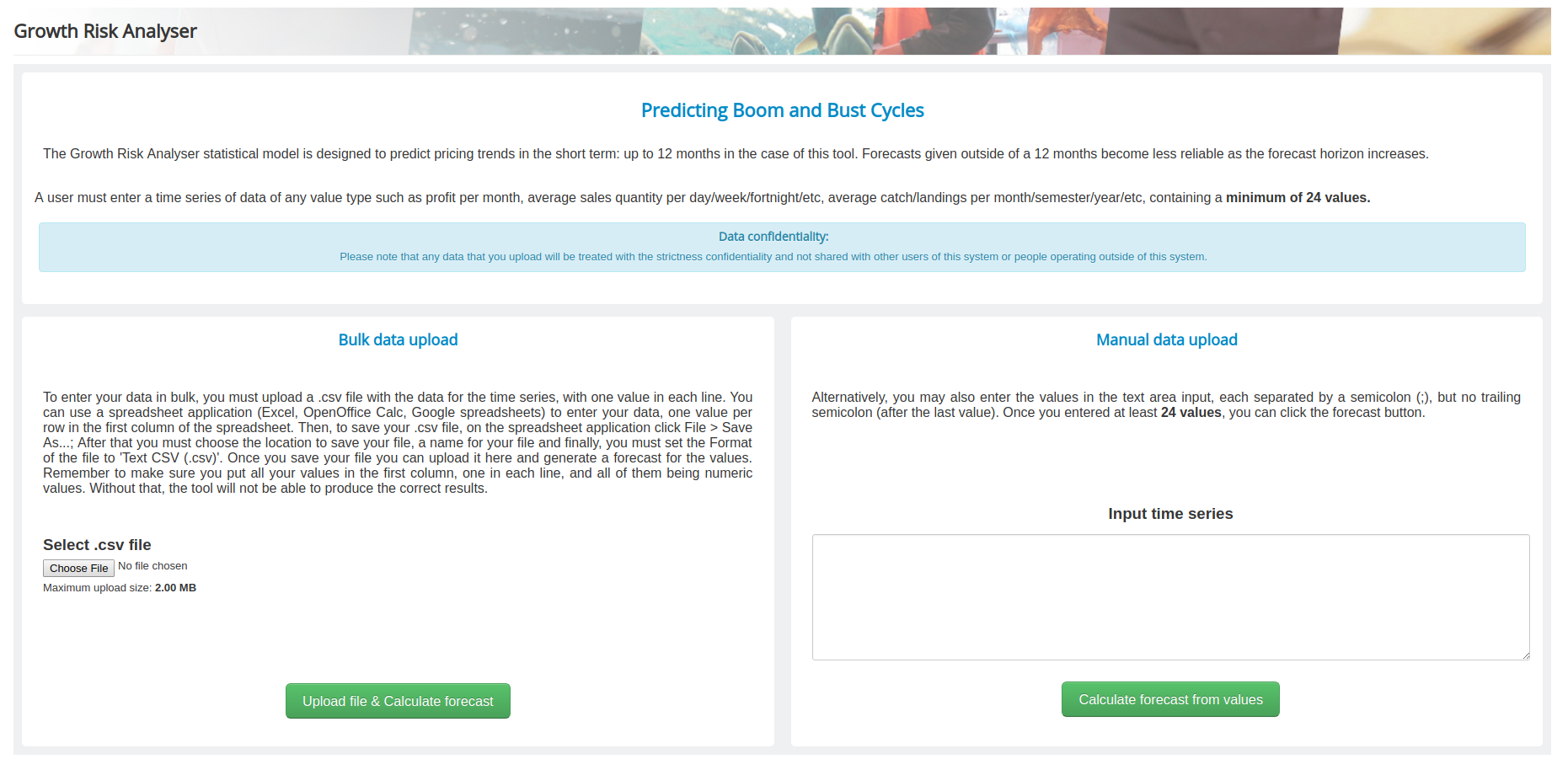
The tool is very simple and it's homepage presents the users with two different forms of input for the data to be analysed.
The input on the left allows the user to upload a file with the time series to be analysed. The file MUST be on a .CSV format to ensure compatibility with the forecasting algorithm, containing all the values in the first column, one value per row:
value1
value2
value3
value4
...
Each row represents a time point in the time series. You don't need to enter the month for the values, as each entry is considered a new point value for the month following its preceding value. The results will display the index value of each entry as ordered in the entry data in the X axis starting at 0, and the forecast results will be added as entries at the end of the time series original values.
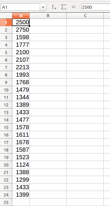
You can create a .CSV file with any spreadsheet editor by simply creating a new spreadsheet and adding the values in the first column, one per row as in the image below:
After that, click the file menu of your spreadsheet editor and select save as.... Once the dialog box for saving opens up, insert the name for the file and select the location. The last and most important and final step is to select Text CSV as a type in the format dropdown for the file type which is generally located above the save button. Once you selected the correct type, click the save button and the file will be ready to be uploaded. You can then proceed to the GRA tool home page and click the choose file button to select your saved file and then click the Upload file and calculate forecast button to generate your forecast. You can download an example .csv file File:Example values.csv.
The input on the left allows you to quickly create a forecast by pasting the values of a time series in the text box and using it as an input. Each value for the time series must be entered one after the other, separated by a semi-colon ;. You will get an error message if any of the values are not in the correct format. Once everything is ready click the calculate button below the input to generate the forecast. You can copy and paste the example below in the tool for a demonstration:
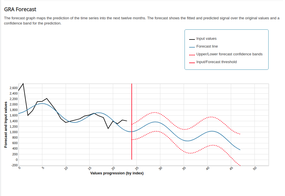
2500;2750;1598;1777;2100;2107;2213;1993;1768;1479;1344;1389;1433;1477;1578;1611;1678;1587;1523;1124;1388;1299;1433;1399
The results
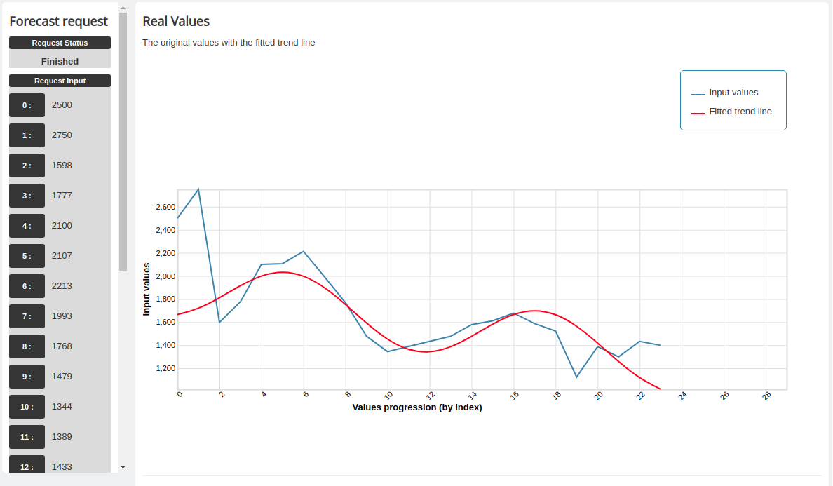
Once you click the forecast button you will be redirected to the results page where you will see on the left sidebar the current request status and the request input as interpreted by the algorithm once the calculations are complete. It may take a few seconds for the algorithm to run, but you should the see the result graphs.
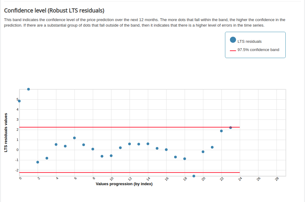
The first graph shows the input values and a fitted trend line for the approximation trend generated. The second graph shows the time series residuals, representing the confidence of the forecast. The more values between the confidence bands, the more accurate will be the results. The last graph will show the original input, the forecast trend line with the forecast values for the next 24 months and the confidence bands. Remember the algorithm is only effective for the first 12 months in its projected confidence, and the further the value goes in the prediction after the 12th value the less accurate is the prediction and should not be considered as having the same forecast confidence.

